Introduction
In the article of Small amplitude oscillations of a double pendulum , the author experimentally investigate a double pendulum model under small angles. By using Tracker to analyze the motion of two pendulum bobs and performing Fourier transformation on their movements, the results can be showed that the motion of bobs can be described as a superposition of two sinusoidal functions with different oscillating modes. Notably, the author mentioned that when the mass of the lower bob is much smaller than that of the upper bob, an exception can occur: the oscillation frequencies of the two modes become approximately equal, leading to the observation of beat phenomena and the energy of one pendulum gradually transferred to the other.
Derive
Assume the length of the two pendulum are $l_1$ 和 $l_2$, the masses of the bobs are $m_1$ 和 $m_2$ and the angle between the vertical are $\theta_1$ 和 $\theta_2$, respectively.
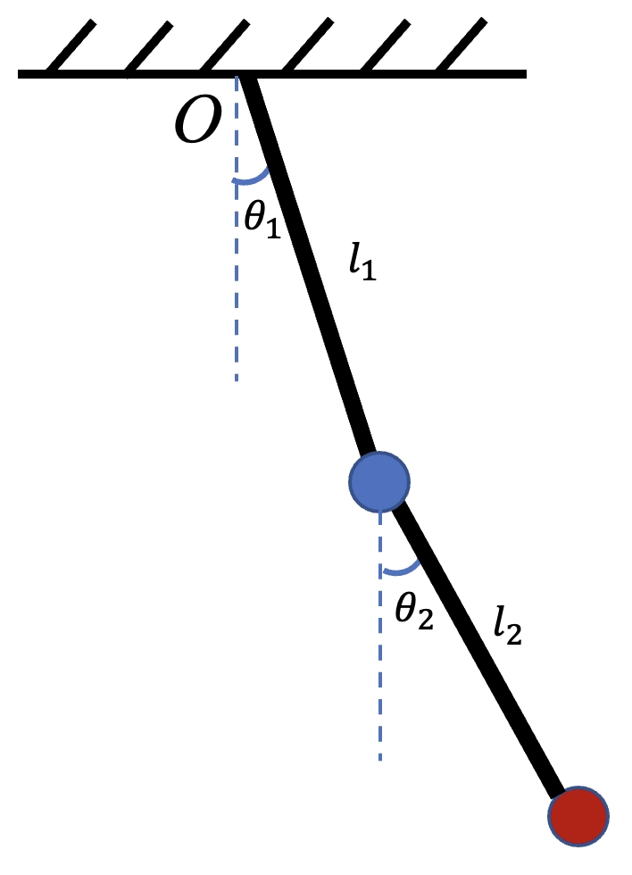
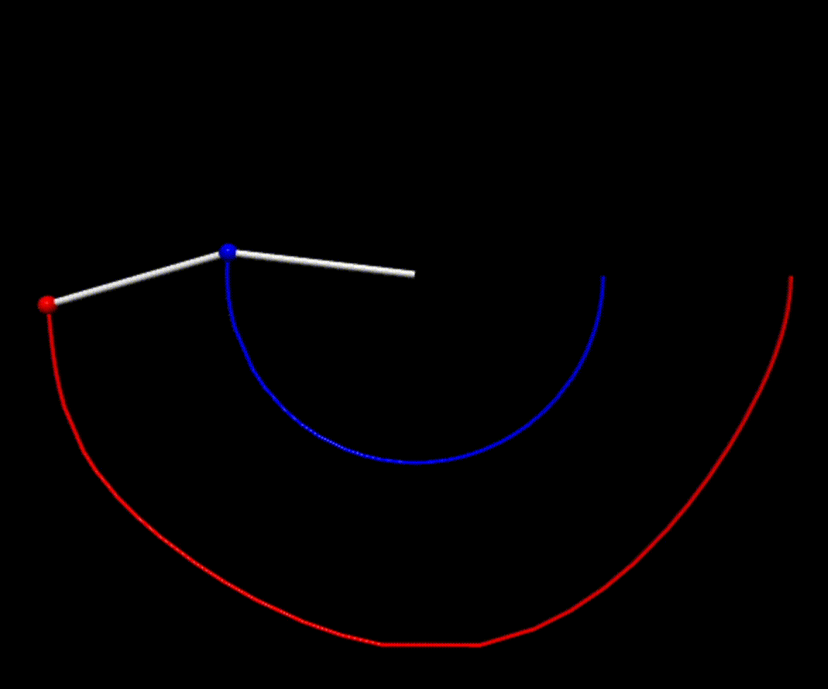
The position of the first bob. $$ x_1 =l_1 sin\theta_1, y_1 =-l_1 cos\theta_1, $$
The position of the second bob. $$ x_2 =x_1+ l_2 sin\theta_2, y_2 =y_1+ l_2 cos\theta_2, $$
The velocity of the first bob. $$ \dot{x_1} =l_1 \dot{\theta_1}cos\theta_1, \dot{y_1} =l_1\dot{\theta_1} sin\theta_1 $$
The velocity of the second bob. $$ \dot{x_2} = \dot{x_1} + l_2 \dot{\theta_2}cos\theta_2, \dot{y_2} =\dot{y_1} + l_2\dot{\theta_2} sin\theta_2 $$
Total kinetic energy of the pendulum bobs system
$$ T= \frac{1}{2}m_1(\dot{x_1}^2+\dot{y_1}^2) + \frac{1}{2}m_2(\dot{x_2}^2+\dot{y_2}^2) $$
Total potential energy of the pendulum bobs system
$$ U = m_1gy_1 + m_2gy_2 $$
Write down the Lagrangian $L = T-V$ of the system and apply it to the Lagrange equations.
$$ \frac{d}{dt}\left( \frac{\partial L}{\partial \dot{\theta_i}} \right) - \frac{\partial L}{\partial \theta_i} = 0 $$
There are two angles $\theta_1$ and $\theta_2$, corresponding to two Lagrange equations. $$ (m_1+m_2)l_1\ddot{\theta_1} + m_2l_2\ddot{\theta_2}cos(\theta_1-\theta_2) + m_2l_2\dot{\theta_2}^2sin(\theta_1-\theta_2)+(m_1+m_2)gsin\theta_1=0 $$
$$ m_2l_2\ddot{\theta_2}+m_2l_1\ddot{\theta_1}cos(\theta_1-\theta_2)-m_2l_1\dot{\theta_1}^2sin(\theta_1-\theta_2)+m_2gsin\theta_2=0 $$
The formula is derived by DeepSeek.
By solving the two equations mentioned above, numerical solutions for $\theta_1$ and $\theta_2$ can be obtained.
Beat Phenomenon
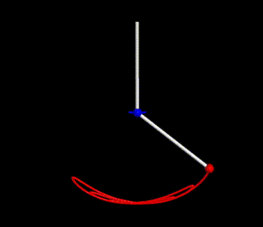
The paper mentions that when the mass of the upper bob $m_1$ is much larger than the mass of the lower bob $m_2$ , the displacements of the two bobs exhibit beat phenomena. Python code is used to simulate this phenomenon. With small initial angles set, the horizontal displacement $x$ of the two bobs against time $t$ is plotted . The masses of the bobs are set as $m_1 = 100$ and $m_2 = 0.1$, the lengths are $l_1=l_2=1$.
The animation is shown in the figure below:
Plot graph of $x_1 - t$、$x_2-t$、$x_1+ x_2-t$ as below.
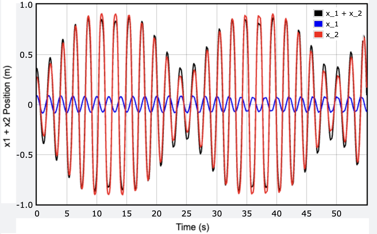
The paper mentions that " the energy in one pendulum is gradually tranferred to the other pendulum." Furthermore, in the animation, it is observed that the amplitude of the lower bob initially increases and then decreases, indicating a change in kinetic energy. The kinetic energy of the upper bob is plotted against time, as shown in the figure below.
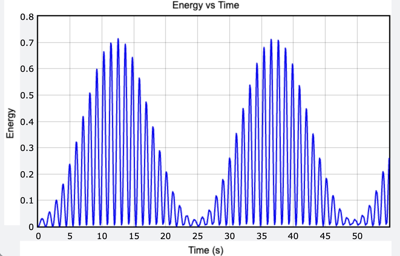
During the motion of two bobs, the kinetic energy transfers between them, exhibiting beat phenomena.
Appendix: Python Code
Python code as below:
Python Code
from vpython import *
import numpy as np
import matplotlib.pyplot as plt
# Parameter settings to observe beats
m1, m2 = 100, 0.1   # Masses, m2 is much smaller than m1 to observe energy transfer effects
theta1, theta2 = np.pi / 36, np.pi / 36 + 0.1  # Make the two mode frequencies close
l1, l2 = 1, 1   # Lengths of the pendulums
g = 9.8  # Gravitational acceleration
# Initial angles
omega1, omega2 = 0.0, 0.0  # Initial angular velocities
dt = 0.01  # Time step
def calc_acc(theta1, theta2, omega1, omega2):
    num1 = -g * (2 * m1 + m2) * np.sin(theta1)
    num2 = -m2 * g * np.sin(theta1 - 2 * theta2)
    num3 = -2 * np.sin(theta1 - theta2) * m2 * (omega2**2 * l2 + omega1**2 * l1 * np.cos(theta1 - theta2))
    den1 = l1 * (2 * m1 + m2 - m2 * np.cos(2 * theta1 - 2 * theta2))
    a1 = (num1 + num2 + num3) / den1
    num4 = 2 * np.sin(theta1 - theta2) * (omega1**2 * l1 * (m1 + m2) + g * (m1 + m2) * np.cos(theta1) + omega2**2 * l2 * m2 * np.cos(theta1 - theta2))
    den2 = l2 * (2 * m1 + m2 - m2 * np.cos(2 * theta1 - 2 * theta2))
    a2 = num4 / den2
    return a1, a2
# VPython scene setup
scene = canvas(title='Double Pendulum - Energy Transfer', width=800, height=600)
anchor = vector(0, 0, 0)
bob1 = sphere(radius=0.05, color=color.blue, make_trail=True)
bob2 = sphere(radius=0.05, color=color.red, make_trail=True)
rod1 = cylinder(radius=0.02, color=color.white)
rod2 = cylinder(radius=0.02, color=color.white)
# Add gplot canvas
graph1 = graph(title="X Position vs Time", xtitle="Time (s)", ytitle="x1 + x2 Position (m)")
curve1 = gcurve(color=color.black, label= "x_1 + x_2")  # Plot x1 + x2 curve
curve_x1 = gcurve(color=color.blue, label = "x_1")
curve_x2 = gcurve(color=color.red,label = "x_2")
graph2 = graph(title="Energy vs Time", xtitle="Time (s)", ytitle="Energy")
curve2 = gcurve(color=color.green)
curve3 = gcurve(color=color.blue)
# Data storage
x2_values = []
time_values = []
t = 0
# Simulation loop
while t < 55:  # Observe for a longer time
    rate(100)
    a1, a2 = calc_acc(theta1, theta2, omega1, omega2)
    omega1 += a1 * dt
    omega2 += a2 * dt
    theta1 += omega1 * dt
    theta2 += omega2 * dt
    pos1 = vector(l1 * sin(theta1), -l1 * cos(theta1), 0)
    pos2 = pos1 + vector(l2 * sin(theta2), -l2 * cos(theta2), 0)
    bob1.pos, bob2.pos = pos1, pos2
    rod1.pos, rod2.pos = anchor, pos1
    rod1.axis, rod2.axis = pos1, pos2 - pos1
    curve1.plot(t, pos1.x + pos2.x)  # Use gcurve to plot x1 + x2 over time
    curve_x1.plot(t, pos1.x)
    curve_x2.plot(t, pos2.x)
    v1 = l1 * omega1
    v2_squared = (l1 * omega1)**2 + (l2 * omega2)**2 + 2 * l1 * l2 * omega1 * omega2 * np.cos(theta1 - theta2)
    v2 = np.sqrt(v2_squared)
    # kinetic energy
    E1 = 0.5 * m1 * v1**2 #+ m1 * g * height1 #green
    E2 = 0.5 * m2 * v2**2 #+ m2 * g * height2 #blue
    # curve2.plot(t, E1)
    curve3.plot(t, E2) #blue
    t += dt
Notice: The VPython library must be installed to run the code above.
Acknowledgments: We thank Rod Cross for his paper; we also thank DeepSeek and ChatGPT for the contributions to the code and formula derivations.