介绍
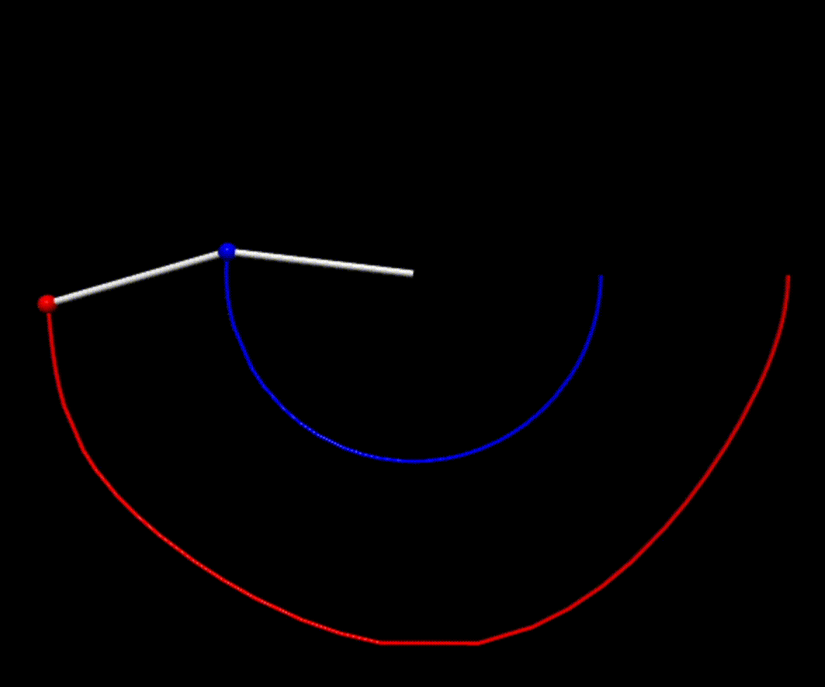
在 Small amplitude oscillations of a double pendulum 一文中,作者实验了小角度下的双摆模型,用 Tracker 软件分析两个摆球的运动,对两球的运动进行傅立叶分析,得到两球的运动可以由两个正弦函数叠加而成。值得一提的是,作者提到,当下摆球的质量远小于上摆球的质量时,可能会出现一种特殊的现象,两种模式的振荡频率大致相同,从而能观察到拍频现象,一个摆的能量会逐渐转移到另一个摆。
An exception can occur if the lower mass is much smaller than the upper mass and then the two modes oscillate at about the same frequency, in which case beating is observed where the energy in one pendulum is gradually tranferred to the other pendulum.
推导
假设摆线长度为 $l_1$ 和 $l_2$,摆球的质量为 $m_1$ 和 $m_2$,摆线与竖直方向的夹角分别为 $\theta_1$ 和 $\theta_2$。
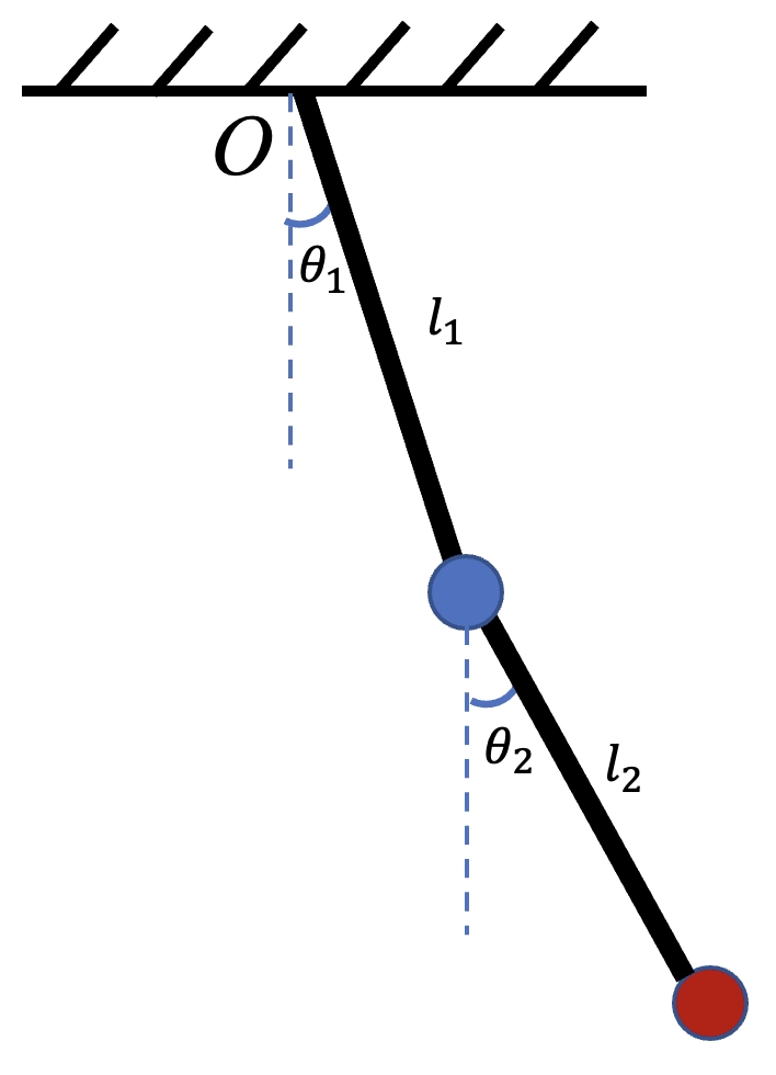
第一个摆球位置 $$ x_1 =l_1 sin\theta_1, y_1 =-l_1 cos\theta_1, $$
第二个摆球位置 $$ x_2 =x_1+ l_2 sin\theta_2, y_2 =y_1+ l_2 cos\theta_2, $$
第一个摆球的速度 $$ \dot{x_1} =l_1 \dot{\theta_1}cos\theta_1, \dot{y_1} =l_1\dot{\theta_1} sin\theta_1 $$
第二个摆球的速度 $$ \dot{x_2} = \dot{x_1} + l_2 \dot{\theta_2}cos\theta_2, \dot{y_2} =\dot{y_1} + l_2\dot{\theta_2} sin\theta_2 $$
写出系统的总动能
$$ T= \frac{1}{2}m_1(\dot{x_1}^2+\dot{y_1}^2) + \frac{1}{2}m_2(\dot{x_2}^2+\dot{y_2}^2) $$
系统总势能
$$ U = m_1gy_1 + m_2gy_2 $$
写出系统的拉格朗日量 $L = T-V$,应用于拉格朗日方程
$$ \frac{d}{dt}\left( \frac{\partial L}{\partial \dot{\theta_i}} \right) - \frac{\partial L}{\partial \theta_i} = 0 $$
角度 $\theta_i$ 有两个 $\theta_1$,$\theta_2$,有两个拉格朗日方程。
$$ (m_1+m_2)l_1\ddot{\theta_1} + m_2l_2\ddot{\theta_2}cos(\theta_1-\theta_2) + m_2l_2\dot{\theta_2}^2sin(\theta_1-\theta_2)+(m_1+m_2)gsin\theta_1=0 $$
$$ m_2l_2\ddot{\theta_2}+m_2l_1\ddot{\theta_1}cos(\theta_1-\theta_2)-m_2l_1\dot{\theta_1}^2sin(\theta_1-\theta_2)+m_2gsin\theta_2=0 $$
通过求解上述两个方程,可以得到 $\theta_1$ 和 $\theta_2$ 的数值解。
拍频现象
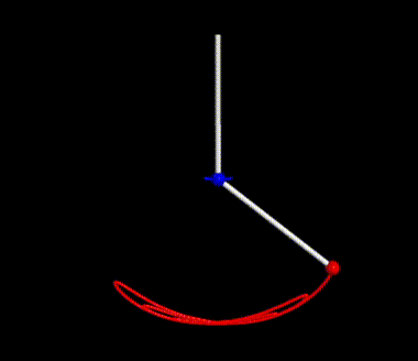
在论文中提到,当上摆球 $m_1$ 的质量远大于下摆球质量 $m_2$,两小球的位移和会出现拍频现象,使用 Python 代码来模拟该现象。设定初始角度较小,绘制两个摆球水平方向$x$ 位移和时间关系图。设置摆球质量 $m_1 = 100$, $m_2 = 0.1$,摆线长度 $l_1=l_2=1$。
动画效果如下图所示:
绘制两球 $x_1 - t$、$x_2-t$、$x_1+ x_2-t$ 的图像,如下图所示。
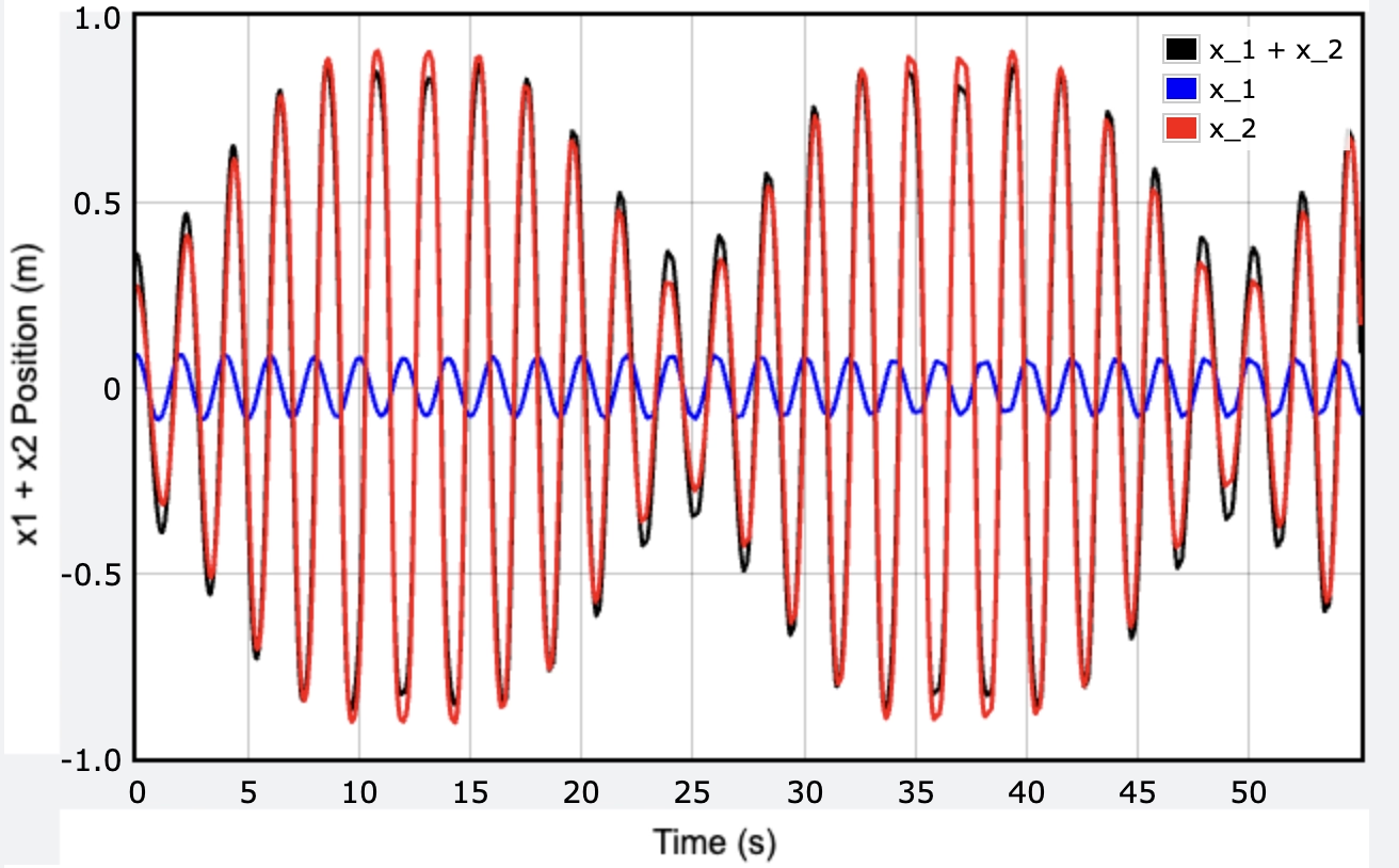
论文中提到“一个摆的能量会逐渐转移到另一个摆”,而且在动画中发现,下摆球的振幅加快,而后减小,即动能会有所变化,绘制上摆球的动能随着时间的图像,如下图所示。
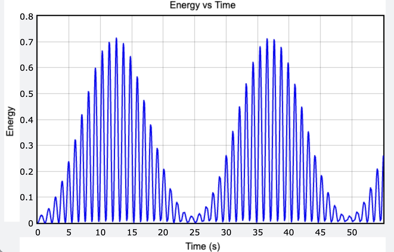
在两球运动中,动能会有所转移,呈现出拍现象。
附录:Python 代码
Python 代码如下:
Python代码
from vpython import *
import numpy as np
import matplotlib.pyplot as plt
# Parameter settings to observe beats
m1, m2 = 100, 0.1   # Masses, m2 is much smaller than m1 to observe energy transfer effects
theta1, theta2 = np.pi / 36, np.pi / 36 + 0.1  # Make the two mode frequencies close
l1, l2 = 1, 1   # Lengths of the pendulums
g = 9.8  # Gravitational acceleration
# Initial angles
omega1, omega2 = 0.0, 0.0  # Initial angular velocities
dt = 0.01  # Time step
def calc_acc(theta1, theta2, omega1, omega2):
    num1 = -g * (2 * m1 + m2) * np.sin(theta1)
    num2 = -m2 * g * np.sin(theta1 - 2 * theta2)
    num3 = -2 * np.sin(theta1 - theta2) * m2 * (omega2**2 * l2 + omega1**2 * l1 * np.cos(theta1 - theta2))
    den1 = l1 * (2 * m1 + m2 - m2 * np.cos(2 * theta1 - 2 * theta2))
    a1 = (num1 + num2 + num3) / den1
    num4 = 2 * np.sin(theta1 - theta2) * (omega1**2 * l1 * (m1 + m2) + g * (m1 + m2) * np.cos(theta1) + omega2**2 * l2 * m2 * np.cos(theta1 - theta2))
    den2 = l2 * (2 * m1 + m2 - m2 * np.cos(2 * theta1 - 2 * theta2))
    a2 = num4 / den2
    return a1, a2
# VPython scene setup
scene = canvas(title='Double Pendulum - Energy Transfer', width=800, height=600)
anchor = vector(0, 0, 0)
bob1 = sphere(radius=0.05, color=color.blue, make_trail=True)
bob2 = sphere(radius=0.05, color=color.red, make_trail=True)
rod1 = cylinder(radius=0.02, color=color.white)
rod2 = cylinder(radius=0.02, color=color.white)
# Add gplot canvas
graph1 = graph(title="X Position vs Time", xtitle="Time (s)", ytitle="x1 + x2 Position (m)")
curve1 = gcurve(color=color.black, label= "x_1 + x_2")  # Plot x1 + x2 curve
curve_x1 = gcurve(color=color.blue, label = "x_1")
curve_x2 = gcurve(color=color.red,label = "x_2")
graph2 = graph(title="Energy vs Time", xtitle="Time (s)", ytitle="Energy")
curve2 = gcurve(color=color.green)
curve3 = gcurve(color=color.blue)
# Data storage
x2_values = []
time_values = []
t = 0
# Simulation loop
while t < 55:  # Observe for a longer time
    rate(100)
    a1, a2 = calc_acc(theta1, theta2, omega1, omega2)
    omega1 += a1 * dt
    omega2 += a2 * dt
    theta1 += omega1 * dt
    theta2 += omega2 * dt
    pos1 = vector(l1 * sin(theta1), -l1 * cos(theta1), 0)
    pos2 = pos1 + vector(l2 * sin(theta2), -l2 * cos(theta2), 0)
    bob1.pos, bob2.pos = pos1, pos2
    rod1.pos, rod2.pos = anchor, pos1
    rod1.axis, rod2.axis = pos1, pos2 - pos1
    curve1.plot(t, pos1.x + pos2.x)  # Use gcurve to plot x1 + x2 over time
    curve_x1.plot(t, pos1.x)
    curve_x2.plot(t, pos2.x)
    v1 = l1 * omega1
    v2_squared = (l1 * omega1)**2 + (l2 * omega2)**2 + 2 * l1 * l2 * omega1 * omega2 * np.cos(theta1 - theta2)
    v2 = np.sqrt(v2_squared)
    # kinetic energy
    E1 = 0.5 * m1 * v1**2 #+ m1 * g * height1 #green
    E2 = 0.5 * m2 * v2**2 #+ m2 * g * height2 #blue
    # curve2.plot(t, E1)
    curve3.plot(t, E2) #blue
    t += dt
备注:需要安装 VPython 库才能运行。
致谢: 感谢 Rod Cross 的论文;感谢 DeepSeek 和 ChatGPT 在代码、公式推导过程中的贡献。